


 15-03-2020, 04:46 PM
 # First calculate the mid prices from the highest and lowest
high_prices = df.loc[:,'High'].as_matrix()
low_prices = df.loc[:,'Low'].as_matrix()
mid_prices = (high_prices+low_prices)/2.0
# Scale the data to be between 0 and 1
# When scaling remember! You normalize both test and train data with respect to training data
# Because you are not supposed to have access to test data
scaler = MinMaxScaler()
train_data = train_data.reshape(-1,1)
test_data = test_data.reshape(-1,1)

| |
|
|
|
15-03-2020, 04:51 PM

  # Train the Scaler with training data and smooth data
smoothing_window_size = 2500
for di in range(0,10000,smoothing_window_size):
    scaler.fit(train_data[di:di+smoothing_window_size,:])
    train_data[di:di+smoothing_window_size,:] = scaler.transform(train_data[di:di+smoothing_window_size,:])

# You normalize the last bit of remaining data
scaler.fit(train_data[di+smoothing_window_size:,:])
train_data[di+smoothing_window_size:,:] = scaler.transform(train_data[di+smoothing_window_size:,:])
  # Reshape both train and test data
train_data = train_data.reshape(-1)

# Normalize test data
test_data = scaler.transform(test_data).reshape(-1)
 # Now perform exponential moving average smoothing
# So the data will have a smoother curve than the original ragged data
EMA = 0.0
gamma = 0.1
for ti in range(11000):
  EMA = gamma*train_data[ti] + (1-gamma)*EMA
  train_data[ti] = EMA

# Used for visualization and test purposes
all_mid_data = np.concatenate([train_data,test_data],axis=0)
15-03-2020, 04:52 PM
15-03-2020, 06:05 PM
15-03-2020, 06:47 PM
15-03-2020, 06:52 PM
window_size = 100
N = train_data.size
std_avg_predictions = []
std_avg_x = []
mse_errors = []
for pred_idx in range(window_size,N):
if pred_idx >= N:
date = dt.datetime.strptime(k, '%Y-%m-%d').date() + dt.timedelta(days=1)
else:
date = df.loc[pred_idx,'Date']
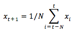
std_avg_predictions.append(np.mean(train_data[pred_idx-window_size:pred_idx]))
mse_errors.append((std_avg_predictions[-1]-train_data[pred_idx])**2)
std_avg_x.append(date)
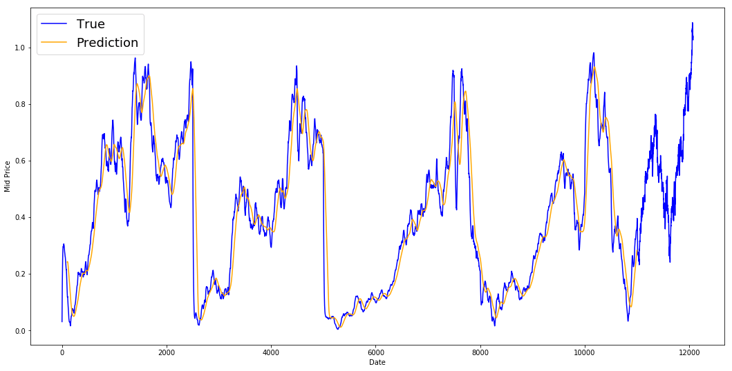
print('MSE error for standard averaging: %.5f'%(0.5*np.mean(mse_errors)))
MSE error for standard averaging: 0.00418
plt.figure(figsize = (18,9))
plt.plot(range(df.shape[0]),all_mid_data,color='b',label='True')
plt.plot(range(window_size,N),std_avg_predictions,color='orange',label='Prediction')
#plt.xticks(range(0,df.shape[0],50),df['Date'].loc[::50],rotation=45)
plt.xlabel('Date')
plt.ylabel('Mid Price')
plt.legend(fontsize=18)
plt.show()
 15-03-2020, 09:16 PM
20-03-2020, 12:52 AM
15-03-2020, 09:16 PM
20-03-2020, 12:52 AM
| الكلمات الدلالية (Tags) |
| إكسبيرت, ورشة, الإصطناعي, الذكاء, برمجة |
| أدوات الموضوع | |
 تعليمات المشاركة
|
لا تستطيع إضافة مواضيع جديدة
لا تستطيع الرد على المواضيع
لا تستطيع إرفاق ملفات
لا تستطيع تعديل مشاركاتك
BB code is متاحة
الابتسامات متاحة
كود [IMG] متاحة
كود HTML معطلة
|


Powered by vBulletin® Version 3.8.11
Copyright ©2000 - 2024, vBulletin Solutions, Inc.
Search Engine Optimisation provided by
DragonByte SEO (Pro) -
vBulletin Mods & Addons Copyright © 2024 DragonByte Technologies Ltd.
جميع المواضيع و الردود المطروحة لا تعبر عن رأي الموقع بل تعبر عن رأي كاتبها وقرار البيع والشراء مسؤليتك وحدك


